
Phytoplankton development at the coastal station "Seebrücke Heiligendamm" in 2015
The Leibniz Institute for Baltic Sea Research conducts a coastal monitoring programme with weekly samplings at the jetty Heiligendamm (54°08,55' N; 11°50,60' E; 300 m off shore, 3 m water depth). The Department of Marine Biology analyses the surface samples, taken by means of a bucket, for phytoplankton composition and biomass and for chlorophyll a.
The phytoplankton biomass is determined by microscopical counting (UTERMÖHL method) and the chlorophyll a concentration by ethanol extraction and fluorometric measurement. Method instructions see http://helcom.fi/action-areas/monitoring-and-assessment/manuals-and-guidelines/combine-manual.
Phytoplankton counting was carried through by use of the counting programme OrgaCount and is based on the HELCOM-biovolume factors which are annually updated: http://www.ices.dk/marine-data/vocabularies/Documents/PEG_BVOL.zip (PEG_BVOL2013; basics see in Olenina et al. 2006). The analytical specifics of the chlorophyll a determination are published by Wasmund et al. (2006). According to the decision of the BLMP-subgroup “Quality Assurance” from 11.9.2008 we show here chlorophyll a data which are not corrected for pheopigments.

Microscopical analysis was not possible in twelve samples as they contained high sediment portions, caused by wind-induced sediment resuspension at the shallow station. The share of sediment-containing samples increased in comparison with the previous year.
The results are shown in Fig. 1.
The phytoplankton biomass was naturally low in January. The development of Mesodinium rubrum, diatoms (Diatomophyceae, particularly Skeletonema marinoi) and Dictyochophycea (Dictyocha speculum, Verrucophora farcimen; here counted as „Chrysophyceae“) started already at the temperature minimum of 2.2°C on 3.2.2015 (Week 5). In contrast to the previous years, Ceratium tripos did not show up at this time.
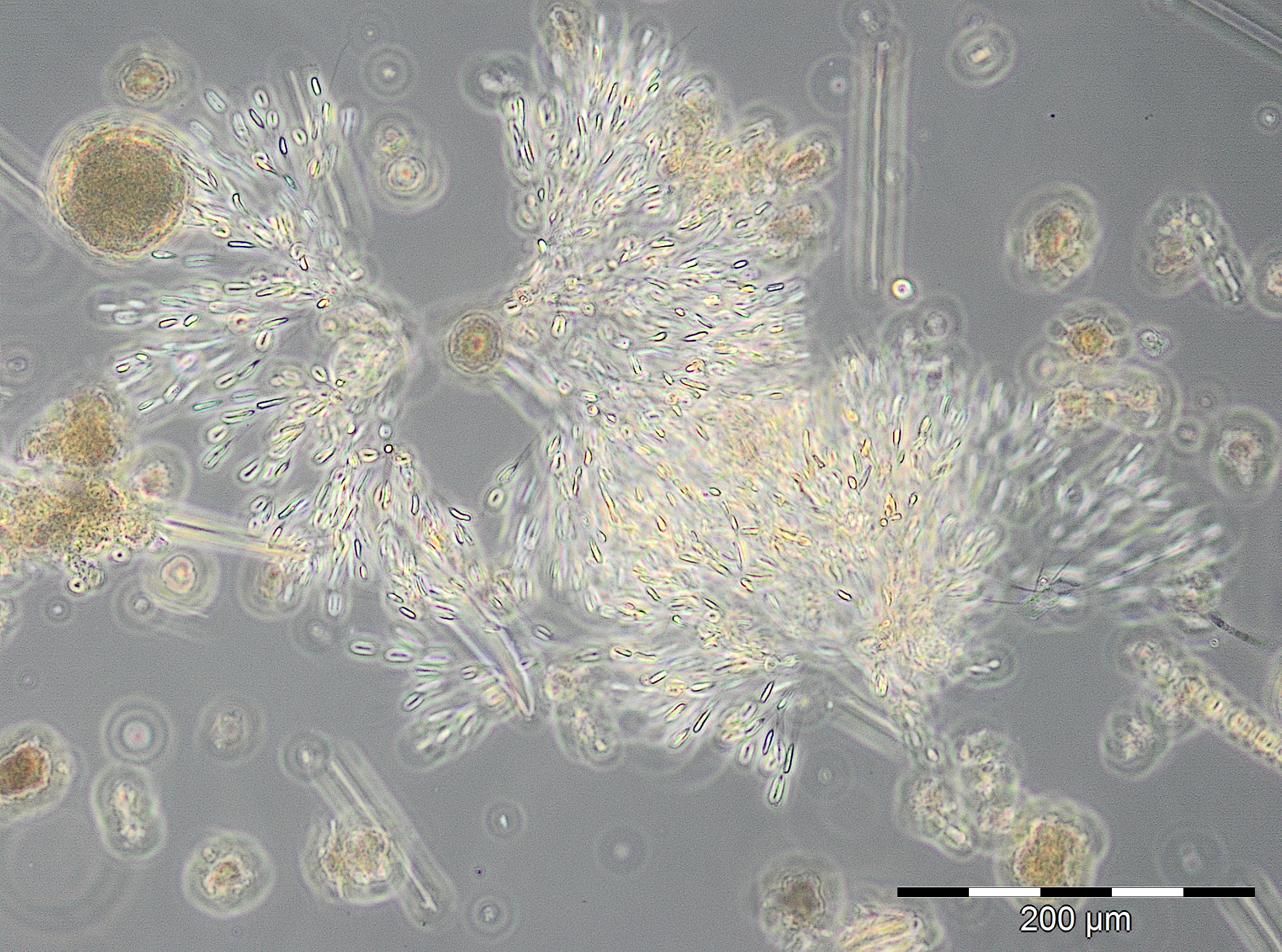
A typical bloom of Skeletonema marinoi (1926 mg/m³, Image 1), accompanied by Dictyocha speculum, developed by 24.2.2015 (Week 8), which is nicely reflected in the chlorophyll-a concentrations.
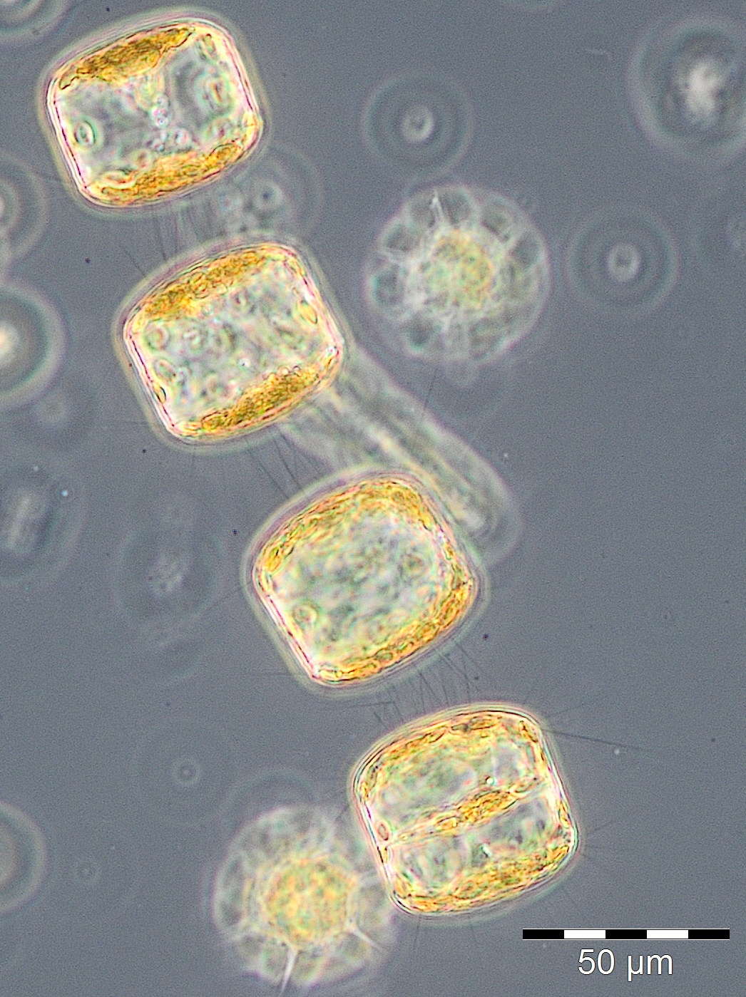
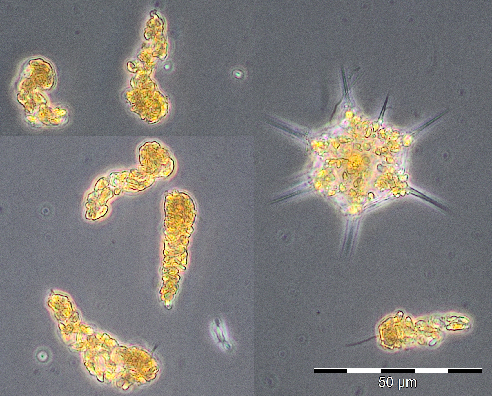
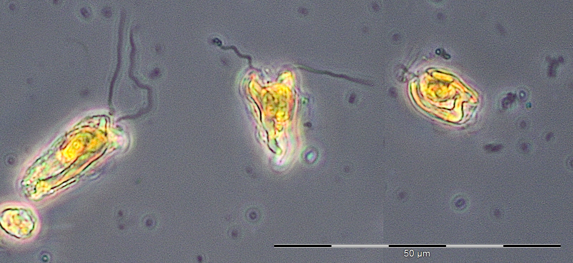
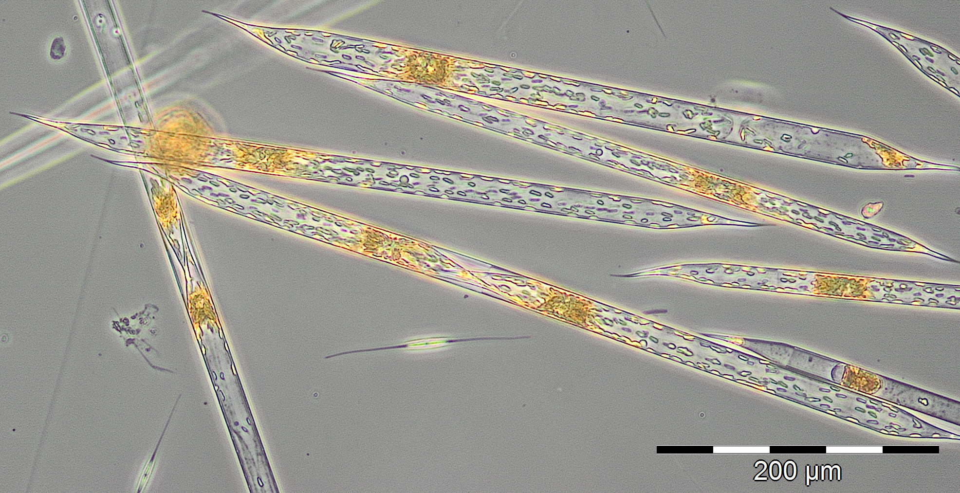
A water body of higher salinity (13.3-16.9 psu) reached the station on 10.3. and 17.3.2015 (Week 10+11). It was dominated by Dictyocha speculum and Verrucophora farcimen (Image 2), which were assigned to Chrysophyceae in Fig.1. Accompanying taxa were diatoms (Rhizosolenia setigera, Proboscia alata, Porosira glacialis see Image 3), dinoflagellates (Peridiniella danica, Gyrodinium spirale) and unidentified Prymnesiophyceae (Image 4).
The water body of higher salinity was drifted away by 24.3.2015 (Week 12) and replaced by a water body of lower salinity (9.7 psu) with Skeletonema marinoi (1663 mg/m³) and Mesodinium rubrum. Again a water body of higher salinity followed on 7.4.2015 (Week 14; 15,5 psu), which was characterized by an unusually high biomass of unidentified Prymnesiophyceae. Also the nice Chrysophyceae Dinobryon balticum is worth mentioning (Image 5).
Consequently, the spring bloom from 2015 was basically a typical diatom bloom. Changes in the species composition within the spring bloom may wrongly be considered a natural succession. In reality it was a sequence of different water bodies passing the station. The low-saline water was characterized by Skeletonema marinoi and Mesodinium rubrum; the high-saline water contained diverse flagellate groups.
After a three-weeks data gap, the phytoplankton biomass was very low in May 2015. The biomass increased slowly in the course of the summer and the phytoplankton became more diverse, with unidentified small Prymnesiales, Gymnodiniales and Cryptophyceae (Plagioselmis, Teleaulax). The typical dinoflagellate of autumn, Ceratium tripos, started its development. On 11.8.2015 (Week 32), the Euglenophyceae Eutreptiella sp. appeared spontaneously. Nitrogen-fixing cyanobacteria stayed very low and also a diatom summer bloom could not be found.
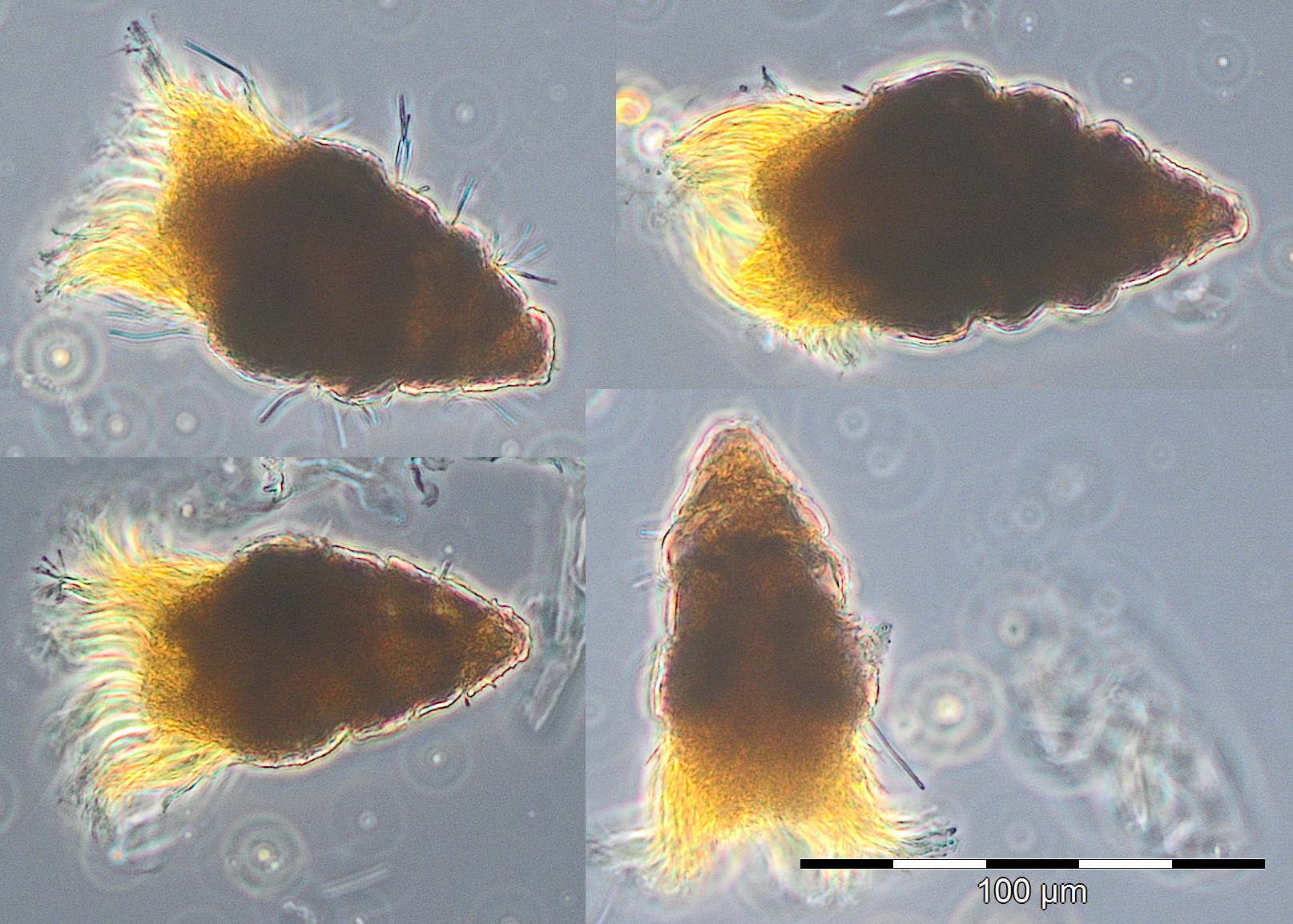
An autumn bloom of diatoms developed by 15.9.2015 (Week 37), mainly composed of Pseudosolenia calcar-avis (Image 6; 863 mg/m³), Cerataulina pelagica (149 mg/m³), Dactyliosolen fragilissimus (55 mg/m³) and Coscinodiscus granii (23 mg/m³). The share of the latter two increased strongly by the next sampling date. Some further diatom species appeared like the typical spring species Skeletonema marinoi from 20.10.-3.11.2015 with biomasses up to 80 mg/m³. Thereafter became important: Rhizosolenia setigera (226 mg/m³) and Guinardia delicatula (79 mg/m³) on 3.11.2015 (Week 44) as well as Actinocyclus sp. (858 mg/m³) on 17.11.2015 (Week 46). Interesting species were also: Polykrikos schwartzii (76 mg/m³) and Laboea strobila (76 mg/m³) on 27.10.2015 and Heterosigma akashiwo (74 mg/m³) on 17.11.2015.
The long-term comparison revealed that the spring bloom was distinct in 2015 in contrast to the untypical spring in 2013. However, a summer bloom typically made by diatoms (like in 2014) or sometimes by cyanobacteria (like in 2013) was definitely not developed in 2015. The characteristic dinoflagellate Ceratium failed in autumn 2015. Instead, the autumn bloom was composed of diverse diatom species. However, the typical diatom Coscinodiscus granii, originating from the Baltic Proper, was only weakly developed with biomasses up 198 mg/m³ which is an indication that outflows from the Baltic Sea were rare in autumn 2015.
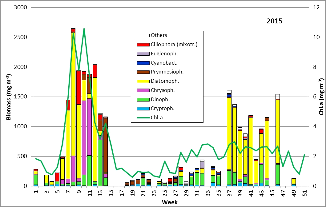
Fig. 1: Composition of the phytoplankton biomass and concentration of chlorophyll a from 6.1. to 22.12.2015 at the jetty Heiligendamm
Acknowledgement
We thank the colleagues of the department Marine Chemistry for their cooperation and especially the colleagues of the department Biological Oceanography, Regina Hansen, Anja Hansen and Annett Grüttmüller, for their participation in the sampling activities. We acknowledge also the technical conditions for the data work and the loading of this report to the IOW site by Solvey Hölzel, Dr. Steffen Bock und Dr. Susanne Feistel.
References:
Olenina, I., Hajdu, S., Andersson, A.,Edler, L., Wasmund, N., Busch, S., Göbel, J., Gromisz, S., Huseby, S., Huttunen, M., Jaanus, A., Kokkonen, P., Ledaine, I., Niemkiewicz, E. (2006): Biovolumes and size-classes of phytoplankton in the Baltic Sea. Baltic Sea Environment Proceedings No.106, 144pp.
http://www.helcom.fi/Lists/Publications/BSEP106.pdf
Wasmund, N., Topp, I., Schories, D. (2006): Optimising the storage and extraction of chlorophyll samples. Oceanologia 48: 125-144.
IOW, 14.05.2016
Dr. Norbert Wasmund,
Susanne Busch,
Christian Burmeister.
Leibniz Institute for Baltic Sea Research Warnemünde (IOW),
Seestr. 15,
D-18119 Rostock-Warnemünde
Corresponding author: Dr. Norbert Wasmund
State of the Baltic Sea
- Annual Reports on the state of the Baltic Sea Environment
- Cruise Reports
- Data from the autonomous measuring stations
- Development of the suboxic and anoxic regions since 1969
- Baltic Thalweg transect since 2014
- Algal blooms at Heiligendamm since 1998
- "Major Baltic Inflow" December 2014
- "Major Baltic Inflow" January 2003
- Baltic saline barotropic inflows 1887 - 2018
- Further Reading
